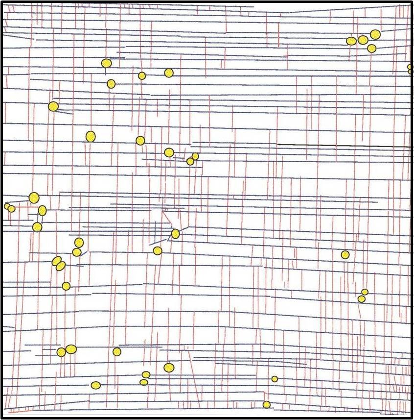
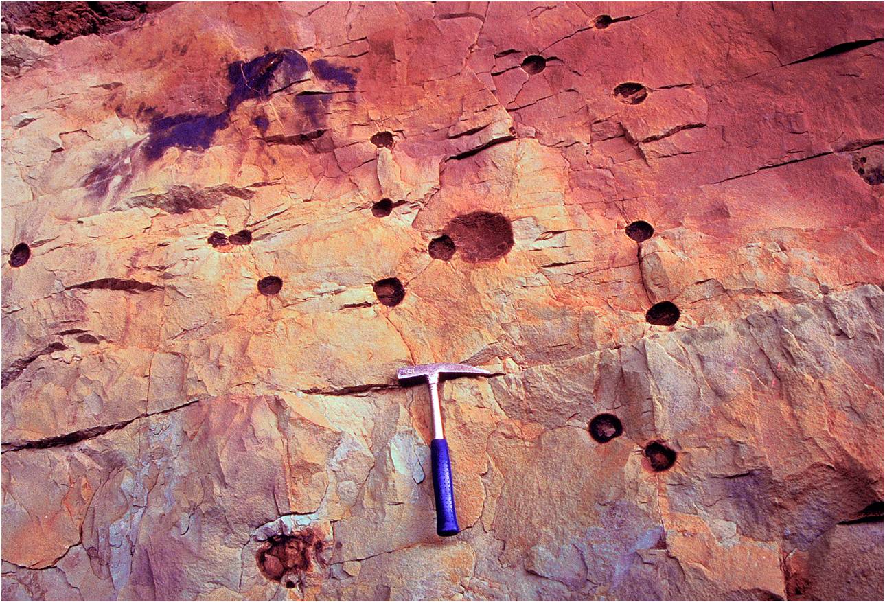
The most common explanation of orthogonal joint patterns described under the link, 'Orthogonal Joint Sets,' is the sequential formation of the two sets in response to a switch (or flip-flop) in the relative magnitudes of the remote principal stresses. For example, the orthogonal joint pattern in Figure 1 was produced in the laboratory by two-stage bending of a glass plate with distributed air bubbles by H. Wu (personal communication). See 'Mechanisms and Mechanics of Joint Domains' for other examples of joint patterns produced by four-point bending, for example Rives et al. (2004). Figure 2 shows an analog in a natural rock; a limestone layer with the imperfections created by the removal of numerous chert nodules by a natural process (see 'Initiation of Joints'). We note that the interpretation of the natural example is not unique. However, regardless of the driving stresses, the stress concentration of different magnitudes at the peripheries of the circular impurity is certain.

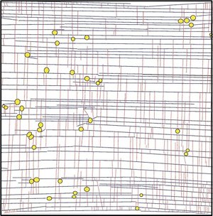Figure 1. Orthogonal joint sets produced in the laboratory by sequential loading. Courtesy of H. Wu.

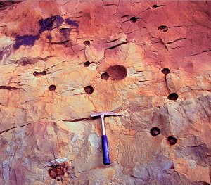Figure 2. Orthogonal joint arrays initiating from spherical flaws controlled in part by the removal of chert nodules from a carbonate rock layer outcropping in Argentinian Patagonia.

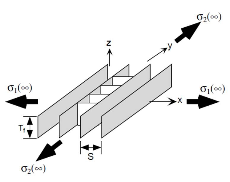
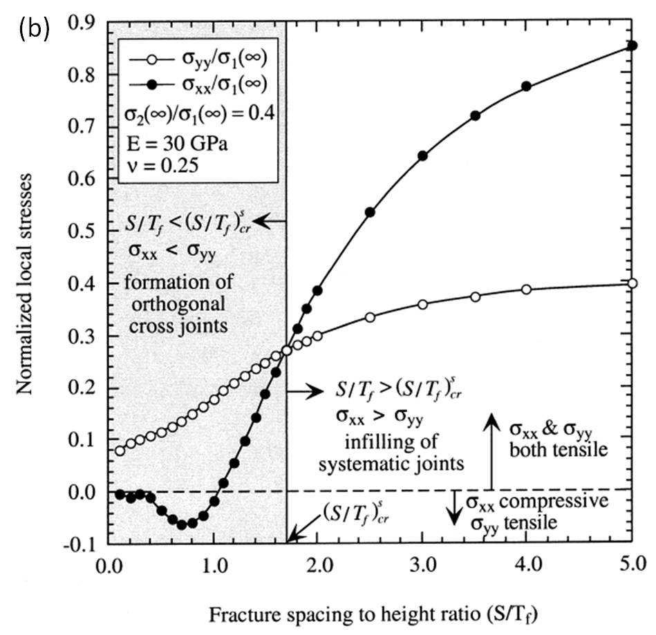
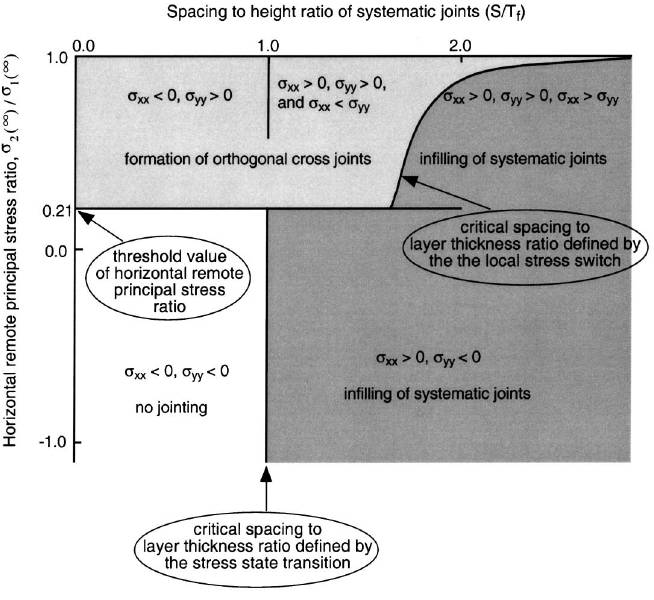
There are other field observations suggesting that in some cases the members of the orthogonal sets have mutually abutting relationships requiring either periodic changes in the relative magnitudes of the remote principal stresses as illustrated by Figures 1 and 2 or a local stress switch under a stationary remote loading as shown schematically by Figure 3. The latter was analyzed by Bai et al. (2002) using numerical models developed by Bai and Pollard. Figure 4 and Figure 5 are diagrams from these studies defining the ranges of particular geometries and stress ratios that would result in the local stress switch thereby leading to the formation of orthogonal joint sets.

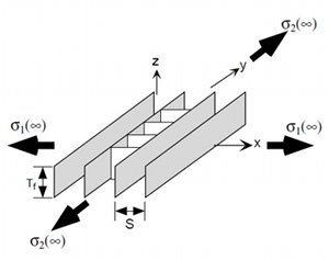Figure 3. Diagram showing the principal stress switch between the two middle fractures as a function of fracture spacing to height ratio, the horizontal principal stress ratio, the vertical stress, Young's modulus, and Poisson's ratio. Slightly changed from Bai et al. (2002).

Figure 4. Formation of orthogonal joints (shaded area) when spacing to height ratio <1.7 of the systematic joints (see Figure 3 for the coordinates and the dimensions). Bai et al. (2002).

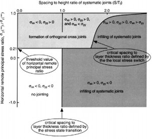Figure 5. Diagram summarizing jointing process under a range of tectonic stresses and their relations to the spacing to layer thickness ratio of the systematic joints. Bai et al. (2002).