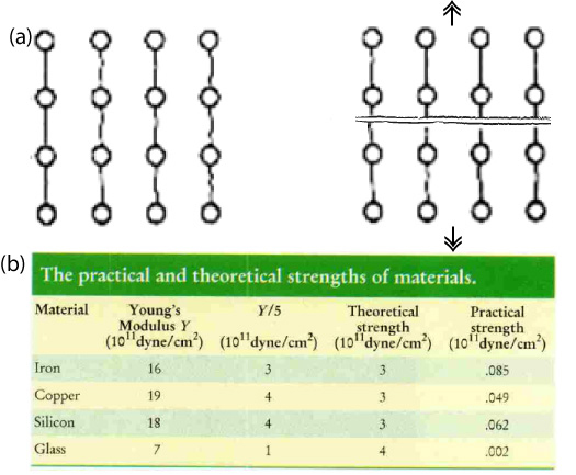
The science of fracture mechanics is concerned with how materials fail by fracture. Ultimately, it aims to predict the fracture of materials under a variety of loading conditions. To this end, the engineering fracture mechanics discipline has made tremendous strides towards achieving this ultimate goal in the past one hundred years. It obviously is beyond the scope of this Knowledgebase to provide a full review of the subject. However, there are so many excellent sources for this purpose. Some of those of which we utilized are Lawn and Wilshaw (1975) in engineering fracture mechanics, and Jaeger et al. (2007), Pollard and Fletcher (2005), and Atkinson (1987) in rock fracture mechanics. For those readers who cannot access these sources for whatever reason, Zehnder's Fracture Mechanics notes (2010) are available through the Internet free of charge for nonprofit educational use. We intend to provide just enough of the subject so that the users of this Knowledgebase have a better understanding of, and appreciation for, the basic premises of fracture mechanics without actually getting into rather complex mathematical details.

The failure strength of a material with a perfect lattice structure (Figure 1a), if such an ideal material exists at all, can be calculated by considering the force needed to overcome the cohesion strength of its atomic bonds. The critical stress thus calculated is known to be about 1/10th (McClintock and Argon, 1966) to 1/5th (Marder and Fineberg, 1996) of the Young's modulus of the material (see the table in Figure 1b).

Figure 1. (a) Schematic illustration of the concept of the theoretical strength of a perfect material based on the force needed to break its atomic bonds. (b) Table showing the theoretical and actual (practical) strength of four common engineering materials along with their Young's moduli. Slightly revised from Marder and Fineberg (1996).

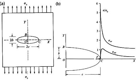
However, laboratory tests on a large variety of materials show that the actual failure stresses are about two orders of magnitude below the calculated theoretical strengths (Figure 1b). This was a dilemma as well as a driving force for a satisfactory explanation of the conflict at the beginning of the 20th century. Finally, a man named Griffith (1920, 1924) provided the answer: He observed that the failure stresses were dependent on the size and orientation of flaws in the laboratory experiments that he conducted using glass rods and spheres. This observation along with the stress concentration models of Inglis (1913) a few years earlier unraveled the paradox of why actual materials have much lower failure stresses than expected. Inglis showed that the stress (σ_yy-stress in y-direction) at the tip of an elliptical hole in a thin plate subjected to remote uniform tension, σ₀, (Figures 2a and b) is proportional to the aspect ratio of the ellipse (c/b) or inversely proportional to the square root of the radius of curvature (ρ) at the ellipse's tips, as expressed by Equation 1.

Equation 1. Stress concentration at the tip of an elliptical hole; b and c are the semi-minor and semi-major axes, respectively, of the ellipse, and ρ is the radius of curvature at its tip. From Ingles (1913).

Figure 2. (a) An elliptical hole with short and long axes of 2b and 2c, respectively, in a thin plate subjected to uniform uniaxial stress. (b) Stresses at the tip of an elliptical hole with c=3b. The problem was originally solved by Inglis in 1913 for a general case; the figures here were taken from Lawn and Wilshaw (1975).

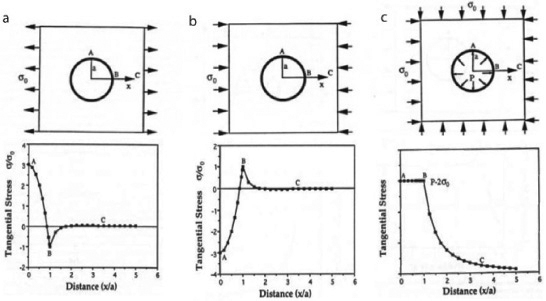
This is known as the stress concentration factor for elliptical flaws. For example, for c=3b, the normalized stresses at the ellipse's tip are plotted in Figure 2b. The stress component in the y-direction (σ_yy at point C) is more than five times the applied stress, σsub#0, and this stress falls off dramatically by a distance equal to about the radius of curvature (ρ) from the tip. Another interesting result is that this stress approaches the background value within a distance of approximately half the major axis of the elliptical flaw. For c=b, the problem is transformed to that of a circular hole in a plate (Figure 3). For a remote load of uniform tension in the x-direction (Figure 3a), the stress amplifications at points A and B are reduced to dimensionless numbers, 3 and -1, respectively, for a remote load of uniform tension. If the applied stress is compressive (Figure 3b), the stress amplifications are -3 and 1, respectively. These results are useful as guidelines in a wide variety of situations. For example, it is possible to produce tensile stress concentrations around flaws even if the remote stress is compressive. Figure 3c shows distribution of the tangential stresses at the periphery of a circular hole with internal fluid or pore pressure, P, in a plate under uniform compressive stresses. The stress at points A and B and any point on the periphery in between is given by P - 2σ₀ (Equation 2), and rapidly declines away from the circular hole. Again, it is possible to have tensile stress at the periphery of pressurized flaws in an environment subjected to compressive confining pressure, depending on the relative magnitude of the internal pressure with respect to the remote stress.

Equation 2. Stress concentration at the periphery of a circular hole subjected to internal pressure, P, and remote uniform stress σ0.

Figure 3. Circular holes in plates subjected to (a) uniform uniaxial tension, (b) uniform uniaxial compression, and (c) hydrostatic compression and internal pressure, P. The lower row shows the the variation of tangential stress between A and B along one quarter of the circles' circumference and at point C, which is far from point B along the x direction. From Aydin (1996).

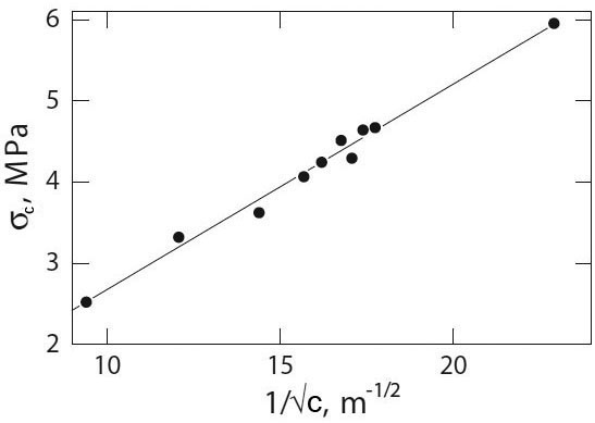
The expression based on the radius of curvature in (Equation 1) captures the unbounded nature of stress at a sharp tip of a discontinuity in a perfectly elastic material; the component of the stress in the y-direction at the tip approaches infinity as the radius of curvature goes to zero. This is often referred to as a stress singularity, and it obviously can never happen in reality because the material around the tip cannot sustain stresses above the yield stress of the material. We will come back to this topic later when we discuss the concept of fracture process zone or fracture tip plasticity.

Griffith went on to propose that the critical failure stress for elastic solids with a certain flaw or a set of flaws under tension can be predicted by considering various forms of energy in play. His energy balance analysis provided that the critical stress, σ_c, for a particular initial fracture (or crack - flaw in his nomenclature) normal to the applied stress (symmetric loading) in a thin plate (plane stress) is inversely proportional to the square root of the half-length of the fracture (Figure 4) as shown in Equation 3. Pulling out the surface energy term (2γ) in Equation 3, which is called the strain energy release rate, fracture extension force, or fracture propagation energy, (G), Griffith proposed that fracture extension will occur when G reaches a critical value G_c for a certain flaw length. It follows that considering multiple flaws, the longest one oriented perpendicular to the applied tensile stress will fail first.

Equation 3. Critical load for failure (plane stress-thin plates) based on Griffith's energy balance analysis. E is the Young's modulus, γ is the surface energy per unit area, and c is the half-length. For plane strain (thick plates), E should be replaced by E / (1 - ν)2 where ν is the Poisson's ration. From Griffith (1924).

Figure 4. Fracture stress vs. the inverse square root of the half crack length. The linear relationship confirms Griffith's major result. Data from Griffith (1920). Figure from Zehnder (2010).

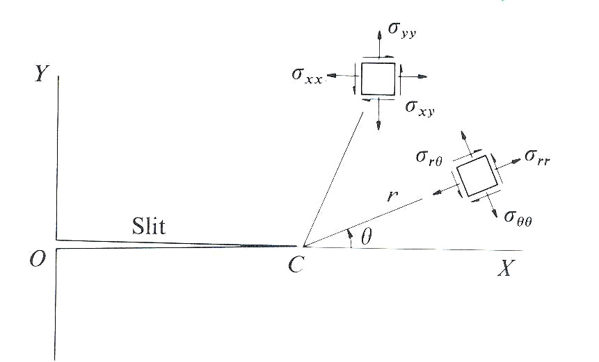
Hence the concept of stress concentration about the so-called Griffith flaw has formed the foundation for the failure process of dominantly brittle materials under tensile loading (other loading conditions will be considered later for shear fractures and closing mode fractures). However, the concept also raised some issues. Griffith did not satisfactorily address the origin of flaws in natural materials, and once the tensile failure loads are reached, there is nothing to stop the incipient flaws from running away unstably since the fracture propagation energy is linearly proportional to the square root fracture half-length. Regarding the former, it is out of the scope of this Knowledgebase to get into the subject of the origin of flaws in engineering materials. We will, however, consider the topic when we deal with initiation of joints, pressure solution seams, and faults in natural rocks, which are the primary focus here. Regarding the latter issue, Irwin (1958) proposed a correctional energy dissipation term to Griffith's energy balance, which requires additional energy input in order for extending a crack by an increment. The physical reasoning for this is the presence of irreversible plastic deformation immediately around the crack tip, called the process zone (see Dugdale-Barenblatt models and a discussion of them by Lawn and Wilshaw, 1975). However, if this zone is small enough with respect to the length of the fracture, the stresses given by equations for various fracture configurations in this section are good outside of the so-called small scale plastic zone (Rice, 1968).

A simple general expression for stresses around a sharp slit-like fracture (Figure 5) in an otherwise homogeneous elastic body is given by Equation 4 (Lawn and Wilshaw, 1975). Here the second part on the right hand side represents the angular (θ) dependence and the first part includes load (K) and distance (r) dependence. Again the local stresses scale with the inverse square root of the distance from the fracture tip and has the inherent stress singularity as this distance vanishes.

Equation 4. Stress distribution (σij) around a slit-like fracture (see Figure 5 for the configuration). K is the stress intensity factor and m takes I, II, and III for modes I, II, and III, respectively. r and θ are distance and angular parameters as defined in Figure 5. From Lawn and Wilshaw (1975).

Figure 5. Diagram illustrating crack tip stress components at a point defined by an angle from the crack plane and a distance to the crack tip in rectangular and polar coordinates. From Lawn and Wilshaw (1975).

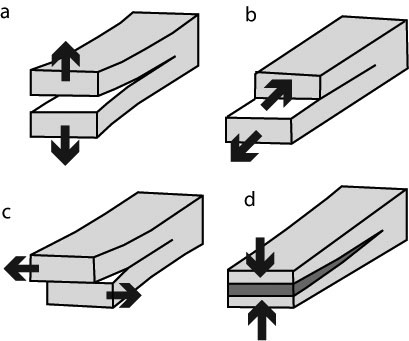
The 'm' in Equation 4 can be I, II, or III, donating three basic modes of fracture mechanics (Figure 6); opening mode, sliding mode, and tearing mode, respectively. In addition, anti-mode I, or closing mode may be added to the three fundamental modes proposed first by Fletcher and Pollard in 1981 (Pollard and Fletcher, 2005), which may be called mode IV just to be consistent with the numerical nomenclature. This will be further discussed under the topic of localized volume reduction structures and pressure solution seams. Here K is the stress intensity factor (K_I, K_II, K_III, for each mode, I, II and III, respectively) and depends on the loading and fracture configuration.

Figure 6. Four modes of fracture: Opening mode (mode I), sliding mode (mode II), and tearing mode (mode III). A fourth mode, closing mode, which is sometimes referred to as anticrack is added to the three modes well-known in engineering fracture mechanics. Redrawn from Lawn and Wilshaw (1975).

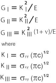
It turns out that the energy release rate for each mode is related to the stress intensity factor for each mode as given by Equation 5 for plane stress. Thus the critical value of the energy release rate for each mode (G_IC, G_IIC, G_IIIC) or the corresponding critical stress intensity factor (K_IC, K_IIC, and K_IIIC), which is called fracture toughness for each mode, are the fracture propagation criteria for each mode for a given material. Fracture toughness is a material property and can be measured by appropriate laboratory tests. Also note that strain energy release rate for different modes are additive.

Equation 5. Relationship between the energy release rate and the stress intensity factor for each fracture mode and the stress intensity factors for plane stress with σyy and σxy being the normal and shear components of the remote stress. Note that E and ν are as defined before. From Lawn and Wilshaw (1975).

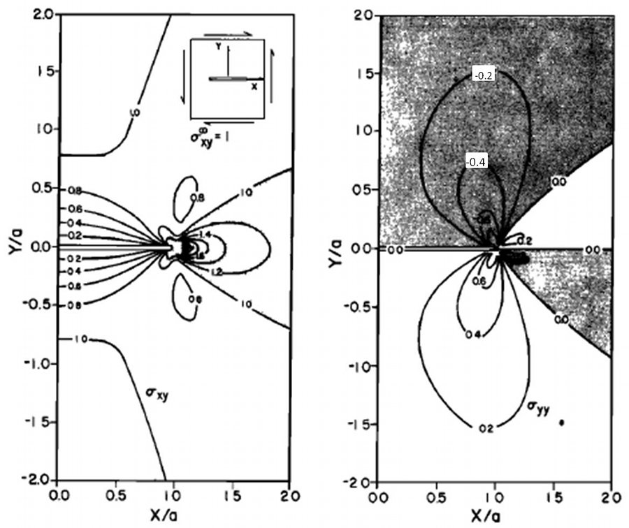
Figure 7 shows the stress distribution around a fracture with a unit half length in an elastic plate subjected to unit pure shear at infinity. The shear stress (σ_xy) is symmetric by the center at x=0 in (7a), and the normal stress (σ_yy) is anti-symmetric about x=0 in (7b). The stresses are different in different regions around the fault, which appear as lobes of various size in the plots. The tip areas are generally characterized by increasing stress concentrations which drop off in some fashion by a distance from the tip, roughly half a length of the shear fracture.

Figure 7. Stress distribution around a single fault within an elastic medium subjected to unit pure shear at infinity. (a) Normalized shear stress (σxy) distribution and (b) normalized normal stress (σyy) distribution. Note that the shaded areas in (b) denote compressive values. From Segall and Pollard (1980).