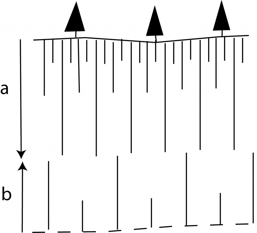
Based on the field data and the mechanical models presented under the related links, it is well-known that columnar joints initiate from the outer boundaries (cooling surfaces) and propagate inward towards the interior. These dual propagation directions commonly result tiers with different cooling rates and consequently, different fracture systems. The most common of the tier systems are two-tier columns (Figure 1), the upper one (entablature or upper colonnade) made up of somewhat irregular, tall and slender columns, while the lower ones (colonnade or lower colonnade) are characterized by highly regular, short and broad columns. The heights of the upper and lower tiers, (a) and (b), respectively, are controlled by the cooling rates in corresponding domains and thicknesses of the flows and have a scaling ratio of about 2:1 to 5:1. Multi-tier columns are also present, especially in thick flows and those flows subjected to quenching by surface waters. The height scaling of these multi-tiers is controlled by the complex thermal regimes responsible for their formations involving the interaction between the geological and hydrological processes and generally are not easily predictable.

Figure 1. Schematic diagram showing two-tiered thermal fracture pattern. (a) and (b) scale with the cooling rates from the top and the base as well as the column bounding fracture interaction.

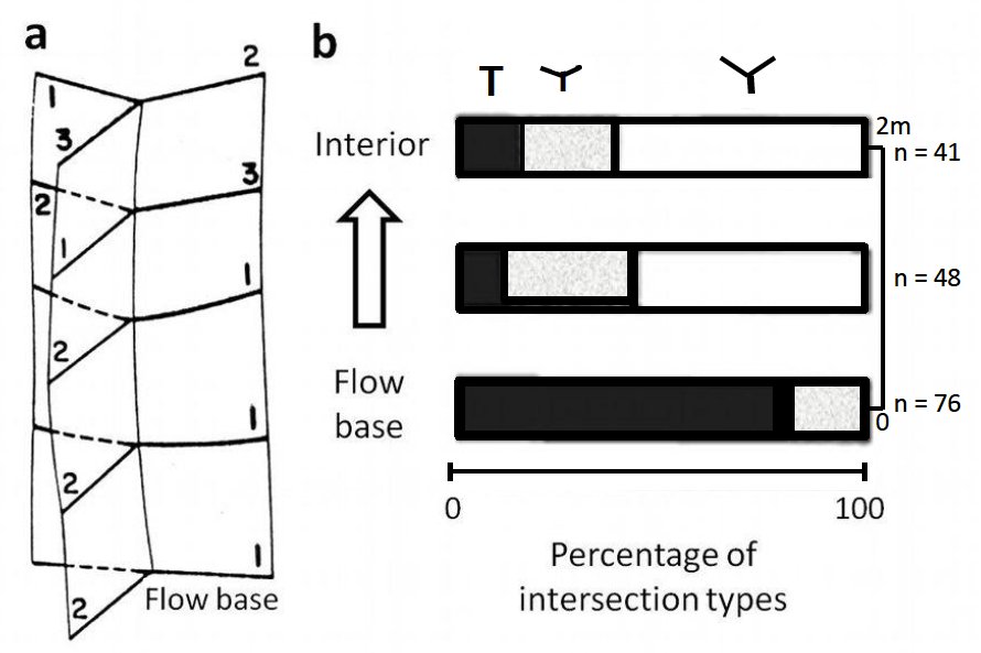
The field data also suggest that, aside from the change of column shapes resulting from the gradual change of intersection angles between laterally and vertically adjacent segments (Figure 2), other dimensions of the growth increments or segments (namely, their heights and widths) also change.

Figure 2. (a, b) Distribution of intersection angles of columnar joints as a function of the distance from cooling boundary surfaces. Orthogonal intersections (T-intersections) are dominant at the boundary surfaces, while the dominant angle approach gradually to a 120 degree (Y-intersection) at the interior, 2m from the surface. The number of measurements at each traverse (n) on the right-hand side. From Aydin and DeGraff (1988).

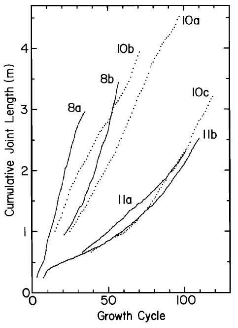
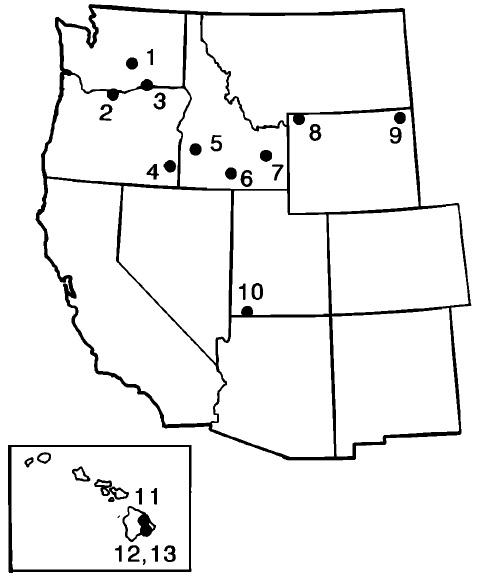
Figure 3 is a plot showing columnar joint lengths (the dimension along the column axes which is commonly vertical) as a function of the number of growth cycles from various locations (see Figure 4 for locations). The general trend and change of slope indicate that the increment heights increase as a function of the fracturing cycle numbers. This is related to the variation of the cooling rate from the cooling boundary towards the interior of the body as will be discussed in other related links.

Figure 3. A plot showing columnar fracture lengths measured along the column axes which are commonly vertical versus cycle (segment) number of cooling surfaces. The curves are concave upward, indicating an increasing segment height towards the interior. From DeGraff and Aydin (1993) and the references therein.

Figure 4. Locations of the field sites for the data in Figures 3 and 5. For specific names, see DeGraff and Aydin (1993).

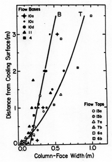
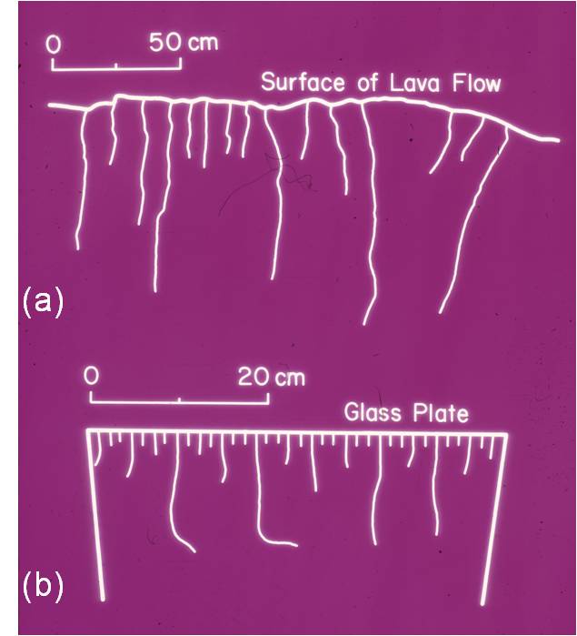
As it is pointed out above, the column size or the spacing of column bounding thermal fractures approximately scales with the inverse of the cooling rate and therefore, the spacing is different for the joint arrays starting from the top and and those started from the base (Figure 5). However, there is another factor, the mechanical interaction of neighboring fractures, which is also important in the evolution of columnar joint spacing (Figure 6). A simple explanation for this can be seen in a model proposed by Lachenbruch (1961;1962) based on the concept of stress relief perpendicular to a vertical joint, which scales with the joint height. Hence, as a system of thermal fractures growing towards the interior of a flow, the spacing would increase as a function of the height of the fractures. Other models, for example, Nemat-Nasser et al, 1980 and DeGraff and Aydin, 1993 that followed Lachenbruch's pioneering work have confirmed his results. In addition, these authors emphasized what is referred to as a fracture elimination process resulting from termination of some fractures and lengthening of others as described under Joint Spacing. Nemat-Nasser et al. (1980) proposed a certain height beyond which the system is stabilized which results in a constant spacing. However, they suggested that several factors, including material heterogeneity may result in a bifurcation from a stationary fracture evolution state.

Figure 5. A plot showing column face width, which is equivalent to joint spacing, from cooling surfaces (top-T and base-B) at the locations marked in Figure 4. Similar to segment height variation, the width also shows an increasing trend by the distance from cooling surfaces. From DeGraff and Aydin (1993) and the references therein.

Figure 6. (a) Spacing of an array of thermal fractures which started from the surface of a lava flow and propagated down towards the interior as seen at a cross section. The spacing is small at or near the top surface and increases towards the interior by the elimination of some of the fractures in the array. From DeGraff (1987). (b) A similar pattern showing a more systematic fracture elimination in a glass plate (unknown source).